Click Start Over menu at the left bottom to start Back to Contents
1. Thoery
A linear transformation on a vector is nothing more than a rotation plus a scaling. For example, in \(\mathbb{R}^2\), we know that the rotation matrix is
\[ \begin{equation} \pmb{A} = \left[\begin{array}{cc} \cos\theta & -\sin\theta \\ \sin\theta & \cos\theta \end{array}\right] \end{equation} \]
and a scale matrix is \(\alpha \pmb{I}\).
Given two sets of normalized orthogonal vectors \(\pmb{v}_1, \pmb{v}_2, \cdots, \pmb{v}_n\) and \(\pmb{u}_1, \pmb{u}_2, \cdots, \pmb{u}_n\), can we find a matrix \(\pmb{A}\) such that
\[ \begin{equation} \pmb{A}\pmb{v}_j = \sigma_j \pmb{u}_j, \; j = 1, \cdots, n \end{equation} \label{Aj} \]
where \(\sigma_j\) are called the singular values.
Eqs. (\ref{Aj}) can be written in a matrix form
\[ \begin{equation} \pmb{A}\pmb{V} = \hat{\pmb{U}}\hat{\pmb{\Sigma}} \end{equation} \label{Amat} \]
where \(\pmb{V} = [\pmb{v}_1, \pmb{v}_2, \cdots, \pmb{v}_n]\), \(\hat{\pmb{U}}=[\pmb{u}_1, \pmb{u}_2, \cdots, \pmb{u}_n]\), and \(\hat{\pmb{\Sigma}} = diag(\sigma_1, \sigma_2, \cdots, \sigma_n)\).
Since \(\pmb{v}_1, \pmb{v}_2, \cdots, \pmb{v}_n\) and \(\pmb{u}_1, \pmb{u}_2, \cdots, \pmb{u}_n\) are normalized orthogonal vectors, \(\pmb{V}\pmb{V}^*=\pmb{I}\) and \(\hat{\pmb{U}}\hat{\pmb{U}}^*=\pmb{I}\). So we find \(\pmb{A}\):
\[ \begin{equation} \pmb{A} = \hat{\pmb{U}}\hat{\pmb{\Sigma}}\pmb{V}^* \end{equation} \label{reducedSVD} \]
Eq. (\ref{reducedSVD}) is called the reduced singular value decomposition of \(\pmb{A}\). In general, we have the following theorem.
Theorem Every matrix \(\pmb{A}\) has a single value decomposition \(\pmb{A}=\pmb{U}\pmb{\Sigma}\pmb{V}^*\).
Single values are unique: \(\sigma_1 \ge \sigma_2 \ge \cdots \sigma_n \ge 0\);
If \(\pmb{A}\) is a square matrix, \(\sigma_j\) are distinct;
\(\pmb{U}\) and \(\pmb{V}\) are unique up to a complex sign.
2. Algorithm
Since
\(\pmb{A}^{*}\pmb{A}=(\pmb{U}\pmb{\Sigma}\pmb{V}^*)^*\pmb{U}\pmb{\Sigma}\pmb{V}^*=\pmb{V}\pmb{\Sigma}^2\pmb{V}^*\),
\(\pmb{A}^{*}\pmb{A}\pmb{V}=\pmb{V}\pmb{\Sigma}^2\).
This implies that \(\pmb{V}\) are the eigenvectors of \(\pmb{A}^{*}\pmb{A}\) associated with eigenvalues \({\Sigma}^2\).
Similarly, since
\(\pmb{A}\pmb{A}^{*}=\pmb{U}\pmb{\Sigma}\pmb{V}^*(\pmb{U}\pmb{\Sigma}\pmb{V}^*)^*=\pmb{U}\pmb{\Sigma}^2\pmb{U}^*\),
\(\pmb{A}\pmb{A}^{*}\pmb{U}=\pmb{U}\pmb{\Sigma}^2\).
This implies that \(\pmb{U}\) are the eigenvectors of \(\pmb{A}\pmb{A}^{*}\) associated with eigenvalues \({\Sigma}^2\).
3. Numerical Examples
Example 1. compute pseudo inverse of a non-full-rank matrix
a <- matrix(c(rep(1, 12), rep(0,9), 1, 1, 1, rep(0,9), 1, 1, 1), 9, 4)
a.svd <- svd(a)
# recover a
a.recover = a.svd$u %*% diag(a.svd$d) %*% t(a.svd$v)
max(abs(a - a.recover))
## [1] 5.551115e-16# determine rank
plot(seq_along(a.svd$d), a.svd$d/sum(a.svd$d))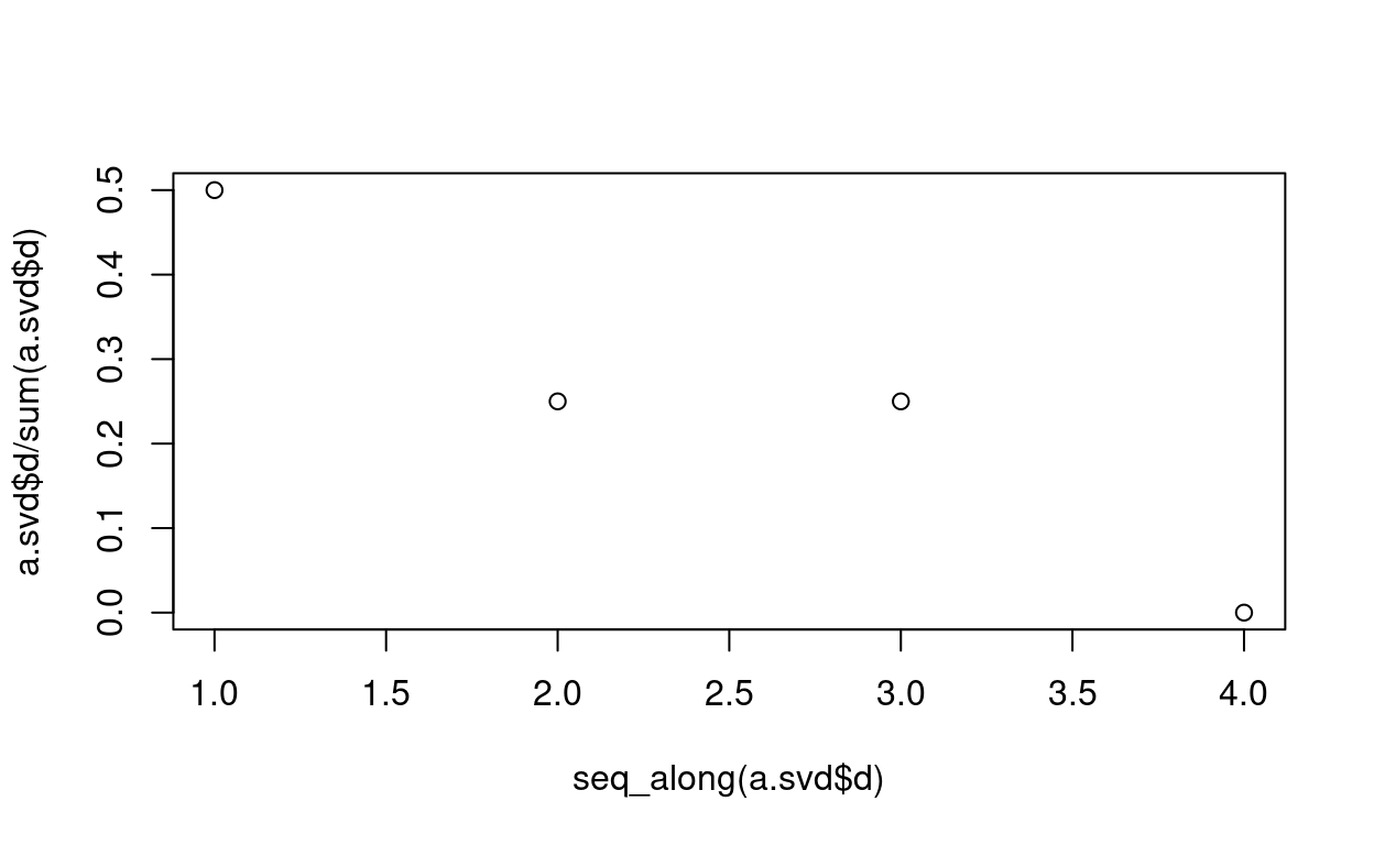
Recover a after truncation according to rank r
r = 3
u.trunc <- a.svd$u[, 1:r]
v.trunc <- a.svd$v[, 1:r]
d.trunc <- a.svd$d[1:r]
# recover a
a.recover.bytrunc = u.trunc %*% diag(d.trunc) %*% t(v.trunc)
max(abs(a - a.recover.bytrunc))
## [1] 6.661338e-16Cumpute pseudo inverse
a.ginv <- v.trunc %*% diag(1/d.trunc) %*% t(u.trunc)
a.ginv
## [,1] [,2] [,3] [,4] [,5] [,6]
## [1,] 0.08333333 0.08333333 0.08333333 0.08333333 0.08333333 0.08333333
## [2,] 0.25000000 0.25000000 0.25000000 -0.08333333 -0.08333333 -0.08333333
## [3,] -0.08333333 -0.08333333 -0.08333333 0.25000000 0.25000000 0.25000000
## [4,] -0.08333333 -0.08333333 -0.08333333 -0.08333333 -0.08333333 -0.08333333
## [,7] [,8] [,9]
## [1,] 0.08333333 0.08333333 0.08333333
## [2,] -0.08333333 -0.08333333 -0.08333333
## [3,] -0.08333333 -0.08333333 -0.08333333
## [4,] 0.25000000 0.25000000 0.25000000