1 Introduction

A biosensor is a device that converts analyte-receptor interaction into detectable signal. Figure 1 describes the operational steps involved in a field-effect transistor based biosensor. A biorecognition element or receptor is immobilized on the transducer surface to recognize analytes or ligands in solution or in the air. The receptor may be an antibody, enzyme, aptamer, peptide, or a cell. The transducer converts analyte-receptor interaction into detectable quantitative electrical or optical signal.

In biosensor design, various properties are considered such as sensitivity, selectivity, stability, reproducibility, regenerability and response time. Among them, the two most important are sensitivity and selectivity. Sensitivity is defined as the smallest concentration of analyte that a biosensor can detect and the shortest response time. Selectivity is defined as the degree of discrimation between the desired analyte and other potential contaminants. In this tutorial, we show some modeling and simulation techniques aiming at designing optimal properties of a biosensor.

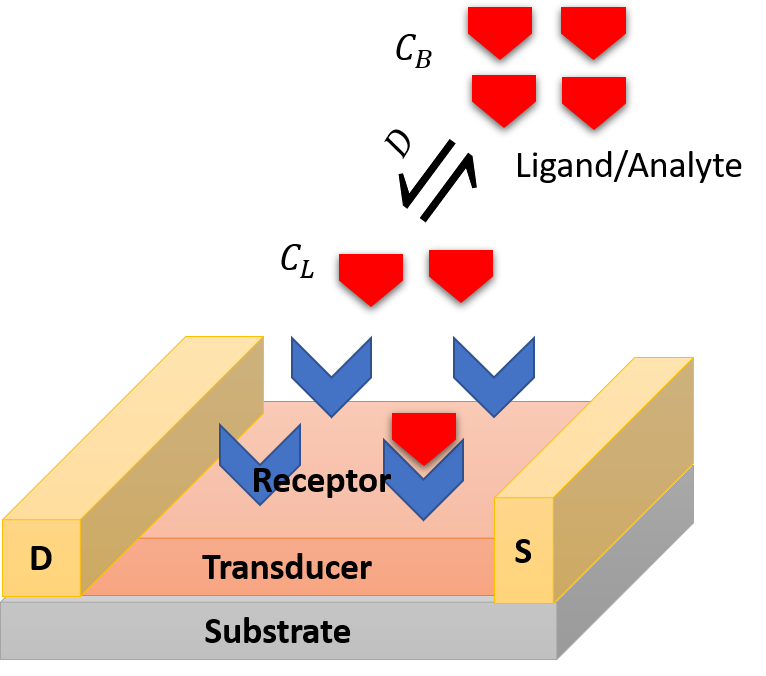
Figure 1: Elementary steps involved in a biosensor.

2 First-Order Reaction Kinetics

Suppose \(C_R^{0}\) is the total undistinguishable binding sites on the surface. \(C_{RL}\) is the occupied binding sites at time \(t\). \(C_{L}\) is available analyte molecules. \(k_a\) and \(k_d\) are the rate of binding to and releasing from a binding site, respectively. The amount balance equation can be written as

\[\begin{equation} C_{RL}(t + \Delta t) = C_{RL}(t) - k_d C_{RL}(t) \Delta t + C_{L} k_a \Delta t (C_{R}^{0} - C_{RL}(t)) \label{eq:eq1} \end{equation}\]

or

\[\begin{equation} \frac{C_{RL}(t)}{dt} = -( k_a C_{L} + k_d) C_{RL}(t) + C_{L} C_{R}^{0} k_a \label{eq:eq2} \end{equation}\]

At equilibrium, Equation (\ref{eq:eq2}) becomes

\[\begin{equation} K_D \equiv \frac{k_d}{k_a} = \frac{C_L (C_{R}^{0} - C_{RL})}{C_{RL}} \label{eq:eq3} \end{equation}\]

Since the initial \(C_{RL}(0)\) is zero, Equation (\ref{eq:eq2}) can be analytically solved as

\[\begin{equation} C_{RL}(t) = \frac{k_a C_L C_{R}^{0}}{k_{obs}} (1 - e^{-k_{obs} t}) \label{eq:eq4} \end{equation}\]

or

\[\begin{equation} \theta(t) = \frac{C_{RL}(t)}{C_{R}^{0}} = \frac{C_L }{C_L + K_D} (1 - e^{-k_{obs} t}) \label{eq:eq5} \end{equation}\]

where \(k_{obs}= k_aC_L + k_d\) is referred to the observed rate constant. \(\theta(t)\) is the occupied fraction of binding sites. \(K_D = \frac{k_d}{k_a}\) is the dissociation constant. Smaller \(K_D\) implies bigger \(k_a\). The system is faster to become saturated and the binding sites is easier to become fully occupied as seen in Equation (\ref{eq:eq5}) even for small amount of analyte \(C_L >> K_D\). This implies that a sensitive biosensor has small \(K_D\). \(K_D\) is a very important parameter which relates macroscopic kinetics with microscopic molecular interaction as shown in next section.

3 Binding Free Energy

Consider the reaction

\[\begin{equation} R + L \rightleftharpoons RL \label{eq:eq6} \end{equation}\]

At equilibrium, according to the equilibrium equation

\[\begin{equation} \mu_{R}^0 + kT\ln\left(\frac{C_R}{c^{\ominus}}\right) + \mu_{L}^{0} + kT\ln \left(\frac{C_L}{c^{\ominus}}\right) = \mu_{RL}^{0} + kT\ln \left(\frac{C_{RL}}{c^{\ominus}}\right) \label{eq:eq7} \end{equation}\]

we obtain that

\[\begin{equation} \Delta G = \mu_{RL}^{0} - \mu_{R}^{0} - \mu_{L}^{0} = kT \ln \frac{C_L C_R}{C_{RL}c^{\ominus}} \label{eq:eq8} \end{equation}\]

Comparing with Equation (\ref{eq:eq3}), we obtain the following important equation which makes a bridge between the macroscopic and microscopic world.

\[\begin{equation} \Delta G = kT \ln \frac{K_D}{c^{\ominus}} \label{eq:eq9} \end{equation}\]

where \(c^{\ominus}\) is the standard concentraion \(1 M\).

4 Calculation of Binding Free Energy on a Pure Surface

At very low adsorbate concentration, it is shown that the standard adsorption free energy on a solid surface can be calculated as (Liu 2009)

\[\begin{equation} \Delta G = - RT\ln \frac{C_{RL}}{C_L} \label{eq:liu} \end{equation}\]

According to Boltzmann distribution law,

\[\begin{equation} \frac{C_{RL}}{C_L} = \frac{e^{-\beta F(RL)}}{e^{-\beta F(L)}} \label{eq:liuY} \end{equation}\]

To account for the fluctuation in the binding region and unbinding region, in practice, Eq (\ref{eq:liuY}) is estimated using their average

\[\begin{equation} \frac{C_{RL}}{C_L} = \frac{\left<e^{-\beta F(RL)}\right>_{RL}}{\left<e^{-\beta F(L)}\right>_{L}} \label{eq:liuYA} \end{equation}\]

where \(F()\) is the potential of mean force.

References

Liu, Yu. 2009. “Is the Free Energy Change of Adsorption Correctly Calculated?” Journal of Chemical & Engineering Data 54 (7): 1981–5. https://doi.org/10.1021/je800661q.