1 Abstract

In order to gain physical insight into the work-free energy relation, we describe an exactly solvable model to represent a single-molecule pulling experiment (SMPE). The free energy to switch one state of the system to the other is exactly calculated. We start with reviewing some mathemtical tools.

2 Dirac delta function

Dirac delta function is defined as

\[\begin{equation} \delta (x) = \begin{cases} 0 & \text{if $x\not=0$} \\ \infty & \text{if $x=0$} \end{cases} \label{eq:Dd} \end{equation}\]

and \(\int \delta(x) dx = 1\).

Proposition 2.1. Dirac delta function can be expressed by \(I_{\delta}(x) \equiv \frac{1}{2\pi}\int dk e^{ikx}\).

Proof. For \(x=0\), the integral is divergent, \(I_{\delta}(x) = \infty\). For \(x \not= 0\),

\[ I_{\delta}(x) = \frac{1}{2\pi}\int dk \cos(kx) + \frac{i}{2\pi}\int dk \sin(kx). \]

Since both integrals are over oscillatory functions, \(I_{\delta}(x) = 0\). Moreover,

\[\begin{equation} \int_{-A}^{A} dx I_{\delta} (x) = \frac{1}{\pi}\int dk \frac{\sin kA} {k} = 1 \; \left(\because \int_{0}^{\infty} \frac{\sin t}{t} dt = \frac{\pi}{2}\right) \label{eq:Deltalim} \end{equation}\]

So \(I_{\delta} (x) = \delta(x)\).

3 Fourier transform

Given a function \(f(x)\) satisfying conditions for the existence of the Fourier transform, the Fourier transform is defined as

\[\begin{equation} \tilde{f}(k) = \int dx e^{ikx}f(x) \label{eq:FT} \end{equation}\]

Given the Fourier transformation \(\tilde{f}(k)\), the original function can be calculated by the inverse transform

\[\begin{equation} f(x) = \frac{1}{2\pi}\int dk e^{-ikx}\tilde{f}(k) \label{eq:IFT} \end{equation}\]

Proposition 3.1. If a function \(f(x)\) has a Fourier transformation, then

\[\begin{equation} f(x) = \int dy \delta (x-y) f(y) \label{eq:DeltaID} \end{equation}\]

Equation (\ref{eq:DeltaID}) tells us that \(\delta(x-y)\) is able to select the functional value \(f(x)\) from all the possible value \(f(y)\).

Proof.

\[\begin{equation} \begin{split} f(x) & = \frac{1}{2\pi} \int e^{-ikx} \tilde{f} (k)dk \\ & = \int dk e^{-ikx} \int dy e^{iky}f(y) \\ & = \int dy f(y) \left[ \frac{1}{2\pi} \int dk e^{-ik(x - y)} \right] \\ & = \int dy f(y) \delta(x-y) \end{split} \label{eq:deltaID} \end{equation}\]

Proposition 3.2. Let \(X\) be a random variable, its probability density function \(p(z)\). Then Equation (\ref{eq:deltaID}) tells us that

\[\begin{equation} \begin{split} p(z) & = \int dx \delta(z-x) p(x) = \left< \delta (z - X) \right> \\ & = \frac{1}{2\pi}\int dx p(x) \left( \int dk e^{ik(z-x)} \right) \\ & = \frac{1}{2\pi}\int dk e^{ikz} \left< e^{-ikx} \right> \end{split} \label{eq:prop3.2} \end{equation}\]

Proposition 3.3. Let \(X\) be a random variable, its probability density function \(p_{X}(x)\). Let \(Y = g(X)\). Then

\[\begin{equation} \begin{split} p_{Y}(y) & = \left< \delta (y - Y) \right> \\ & = \left< \delta (y - g(X)) \right> \\ & = \lim_{N\rightarrow\infty} \frac{1}{N}\sum_{n=1}^{N}\delta(y-g(X_n)) \\ & = \int dx \delta(y - g(x)) p_X(x) \end{split} \label{eq:prop3.3} \end{equation}\]

Proposition 3.4. Let \(X\) be a random variable, its probability density function \(p_{X}(x)\). Let \(Y = g(X)\) and g has an inverse function \(h=g^{-1}\). Let \(z = g(x)\). Then \(x = h(z)\) and

\[\begin{equation} \begin{split} p_{Y}(y) & = \int dx \delta(y - g(x)) p_X(x) \\ & = \int dz\left|\frac{dh(z)}{dz}\right|\delta(y - z) p_X(h(z)) \\ & = \left|\frac{dh(y)}{dy}\right|p_X(h(y)) \end{split} \end{equation}\]

4 The SMPE Model

Let us consider a single molecule of mass \(m\) represented by the red sphere in Figure 1. The interaction with a surface is described by a spring force with spring constant \(k\) and equilibrium length \(\xi_{0}\). The sphere is pulled away at a constant velocity \(V\) from the surface in the direction perpendicular to the surface. The pulling force is described by another idential spring. Assuming the potentials are harmonic, the Hamiltonian of the system is readily expressed as (Hı́jar and Zárate 2010)

\[\begin{equation} H(x, p) = \frac{p^2}{2m} + \frac{k}{2}\left[\left(x - \xi_{0}\right)^2 + \left(Vt - (x - \xi_{0})\right)^2\right] \label{eq:Hamil} \end{equation}\]

where \(x\) is the distance of the sphere to the surface, and \(p\) the momentum.

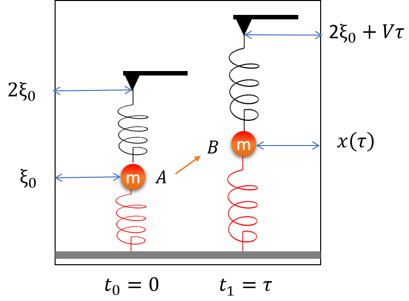
Figure 1: Schematic representation of a single-molecule pulling experiment.

From Hamiltonian (\ref{eq:Hamil}), the equations of motion of the sphere follow:

\[\begin{equation} m\frac{d^2 x}{dt^2} = - 2 k (x - \xi_{0}) + k Vt \label{eq:motion} \end{equation}\]

The general solution to Equation (\ref{eq:motion}) is

\[\begin{equation} x(t) = A_0 \cos(\sqrt{2} \omega t + \theta_0) + \xi_0 + \frac{1}{2}Vt \label{eq:sol} \end{equation}\]

where \(\omega = \sqrt{k/m}\) is the frequency. The amplitude \(A_0\) and phase \(\theta_0\) are determined by initial position \(x_0\) and momentum \(p_0\) at \(t = 0\). Thus they sastify the following equations

\[\begin{equation} x_0 = A_0 \cos(\theta_0) + \xi_0 \label{eq:x0} \end{equation}\]

\[\begin{equation} p_0 = -\sqrt{2} m\omega A_0 \sin(\theta_0) + \frac{1}{2}m V \label{eq:p0} \end{equation}\]

From Equations (\ref{eq:x0}) and (\ref{eq:p0}), we obtain

\[ \cos(\theta_0) = \frac{x_0 - \xi_0}{A_0} \\ \sin(\theta_0) = \frac{\frac{1}{2}m V - p_0}{\sqrt{2} m\omega A_0} \\ A_0 = \left[(x_0 - \xi_0)^2 + \left(\frac{\frac{1}{2}m V - p_0}{\sqrt{2} m\omega}\right)^2\right]^{1/2} \]

Therefore, Equation (\ref{eq:sol}) becomes

\[\begin{equation} x(t) = \xi_0 + \frac{V}{2}t + (x_0 - \xi_0) \cos(\sqrt{2} \omega t) + \\ \frac{\sqrt{2}(2p_0 - mV)}{4 m\omega} \sin(\sqrt{2}\omega t) \label{eq:exactSol} \end{equation}\]

The derivative of \(x(t)\) with respect to \(t\) is

\[\begin{equation} x'(t) = \frac{V}{2} - \sqrt{2} \omega (x_0 - \xi_0) \sin(\sqrt{2} \omega t) + \\ \frac{2 p_0 - mV}{2 m}\cos(\sqrt{2} \omega t) \label{eq:exactSolD} \end{equation}\]

The work \(W\) required to move the particle from its position at \(t = 0\) to its position at time \(t\) is given by the energy difference:

\[\begin{equation} \begin{split} W & = H(x(t), p(t)) - H(x_0, p_0) \\ & = \phi(t) - p_0 \frac{V}{2} (1 - \cos\sqrt{2}\omega t ) - (x_0 - \xi_0) \frac{m\omega V}{\sqrt{2}} \sin\sqrt{2}\omega t \end{split} \label{eq:W} \end{equation}\]

where \(\phi(t)\) is given by

\[\begin{equation} \phi (t) = \frac{m\omega^2}{4} \left[(Vt)^2 + \frac{V^2}{\omega^2}(1 - \cos \sqrt{2}\omega t)\right] \label{eq:phi} \end{equation}\]

5 Viewpoint from classical mechanics

In classical mechanics, we consider \(A\) and \(B\) as two static states (rest states). If we set the initial conditions as

\[ x(0) = \xi_0 \\ \frac{dx(t)}{dt}\mid_{t=0} = 0 \]

We obtain the exact solution to Equation (\ref{eq:motion})

\[\begin{equation} x(t) = -\frac{\sqrt{2}V}{4\omega} \sin(\sqrt{2} \omega t) + \xi_0 + \frac{1}{2}Vt \label{eq:exactSol0} \end{equation}\]

The external force acting on the dummy atom represented by the triangle in Figure 1 is \(f_{ext} = m\omega^2 (2\xi_0 + Vt - x(t) - \xi_0)\). Its trajecotry is \(Vt\). So the external work to stretch the spring from \(x_0\) to \(x_{\tau}\) in time \(\tau\) is

\[\begin{equation} \begin{split} W & = \int_{0}^{\tau} \overrightarrow{F}(t)\cdot \overrightarrow{r}'(t) dt \\ & = mV\omega^2 \int_{0}^{\tau}(\xi_0 + Vt - x(t))dt \\ & = mV\omega^2 \int_{0}^{\tau} (\frac{\sqrt{2}V}{4\omega} \sin(\sqrt{2} \omega t) + \frac{1}{2}Vt)dt \\ & = \frac{m\omega^2}{4}V^2 \tau^2 + \frac{mV^2}{4}(1-\cos\sqrt{2}\omega\tau) \end{split} \label{eq:W1} \end{equation}\]

Equation (\ref{eq:W1}) is exactly the energy difference derived in Equations (\ref{eq:W}) and (\ref{eq:phi}). Correctly calculating the work is critical in applying the work-free energy formula.

6 Viewpoint from statistical thermodynamics

From the viewpoint of statistical thermodynamics, the initial positions \(x_0\) and momenta \(p_0\) of the particle at a given temperature are random variables with the Boltzmann distribution:

\[\begin{equation} \begin{split} f(p_0, x_0) & = \frac{\exp(-\beta H(p_0, x_0))}{\int_{-\infty}^{+\infty}\int_{-\infty}^{+\infty}\exp(-\beta H(p_0, x_0))dp_0dx_0} \\ & = \frac{\beta \omega}{\sqrt{2}\pi} \exp(-\beta (\frac{p_0^2}{2m} + m \omega^2 (x_0 - \xi_0)^2)) \end{split} \label{eq:Boltz} \end{equation}\]

where \(\beta = 1/k_BT\). Using Gaussian integral, we obtain that the average \(<\exp[-iqW]>\) under the distribution \(f(p_0, x_0)\) is

\[\begin{equation} \begin{split} <\exp[-iqW]> & = \int_{-\infty}^{+\infty}\int_{-\infty}^{+\infty}dp_0dx_0exp[-iqW]f(p_0, x_0)\\ & = \frac{\beta \omega}{\sqrt{2}\pi} e^{-iq\phi} \int_{-\infty}^{+\infty}dp_0 \exp\left[-\frac{\beta p_0^2}{2m} + iq\frac{V}{2}p_0 (1-cos(\sqrt{2}\omega t)\right] \times \\ & \int_{-\infty}^{+\infty}dx_0 \exp\left[-\beta m \omega^2 (x_0 - \xi_0)^2 + i q \frac{m \omega V}{\sqrt{2}}(x_0 - \xi_0) \sin(\sqrt{2}\omega t)\right] \\ & = \exp \left[-iq\phi - q^2 \frac{mV^2}{4\beta}(1-cos\sqrt{2}\omega t)\right] \end{split} \label{eq:pq} \end{equation}\]

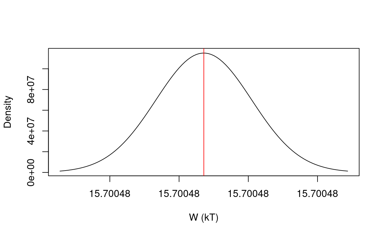
Since work \(W\) is a function of \((p_0, x_0)\), according to Equation (\ref{eq:prop3.3}), the probability density function \(P(w)\) is given by

\[\begin{equation} \begin{split} P(W) & = \frac{1}{2\pi}\int dq e^{iqW} \left< e^{-iqW} \right> \\ & = \frac{1}{2\pi}\int dq \exp \left[iqW -iq\phi - q^2 \frac{mV^2}{4\beta}(1-cos\sqrt{2}\omega t)\right] \\ & = \frac{1}{\sqrt{2\pi}\sigma}\exp\left[-\frac{(W-\phi)^2}{2\sigma^2}\right] \end{split} \label{eq:Wpdf} \end{equation}\]

where the variance \(\sigma^2\) is given by

\[\begin{equation} \sigma^2 = \frac{mV^2(1-\cos\sqrt{2}\omega t)}{2\beta} \label{eq:Wvariance} \end{equation}\]

7 Free energy

The free energy difference of the particle at time \(t=\tau\) and at time \(t=0\) can be easily calculated:

\[\begin{equation} \begin{split} \Delta F & = -k_B T \log \frac{Q(\tau)} {Q(0)} \\ & = -k_B T \log \frac{\int_{-\infty}^{+\infty}dx \exp\left[-\frac{\beta m \omega^2}{2}[(x-\xi_0)^2 + (x- V\tau - \xi_0)^2]\right] } {\int_{-\infty}^{+\infty}dx_0 \exp\left[-\beta m \omega^2 (x_0-\xi_0)^2\right]} \\ & = \frac{1}{4} m \omega^2 V^2 \tau^2 \end{split} \label{eq:freeE} \end{equation}\]

Equation (\ref{eq:Wpdf}) tells us that the mean of the work is

\[ <W> = \phi (t) = \frac{m\omega^2}{4} \left[(V\tau)^2 + \frac{V^2}{\omega^2}(1 - \cos \sqrt{2}\omega \tau)\right] \geq \Delta F \]

The equality holds when \(V\rightarrow 0\), which corresponds to the so-called irriversible processes. However,

\[\begin{equation} \begin{split} <e^{-\beta W}> & = \int e^{-\beta W} P(W) dW \\ & = \frac{1}{\sqrt{2\pi}\sigma}\int dW\exp\left[-\beta W -\frac{(W - \phi)^2}{2 \sigma^2} \right]\\ & = \exp\left[-\beta (\phi - \frac{\beta}{2}\sigma^2)\right]\\ & = \exp[-\beta \Delta F] \end{split} \label{eq:Jz} \end{equation}\]

In general, equality (\ref{eq:Jz}) holds. The equality is called the Jarzynski equality.

8 Example

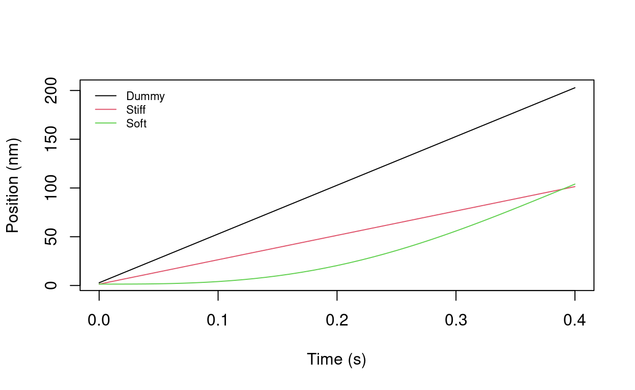
Example 8.1 Let the sphere represent a single peptide with mass \(2\times 10^{-24} kg\). The spring constant is \(65 pN/nm\). The equilibrium length is \(1.4 nm\). The pulling speed is \(500 nm/s\). Assume that its initial position is at \(1.4 nm\) and initial velocity is \(0\).

1. plot the time evolution of the particle and the dummy atom.

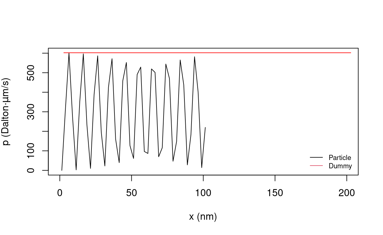
2. Plot the trajectory of the particle and the dummy atom in \((x, p)\) phase space.

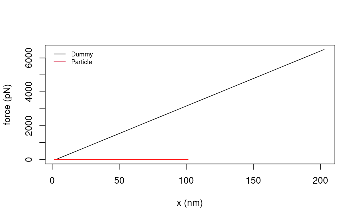
3. Plot the force-extenstion profile of the particle and the dummy atom.

4. Plot work distribution

References

Hı́jar, Humberto, and José M Ortiz de Zárate. 2010. “Jarzynski’s Equality Illustrated by Simple Examples.” European Journal of Physics 31 (5): 1097–1106. https://doi.org/10.1088/0143-0807/31/5/012.