1 Random variable and sample

The familiar random variable \(X\) is the two possible outcomes when we toss a coin. We take two values \(0\) or \(1\) to represent tail or head in the outcome. If the probability that it takes the value \(1\) is \(q\), we have the Bernoulli probability distribution

\[\begin{equation} P(X = x) = q^x (1-q)^{(1-x)} \label{eq:bernoulli} \end{equation}\]

If \(Y\) is the possible number of heads in a total of \(N\) tosses, the probability distribution is given by the Binomial distribution

\[\begin{equation} P(Y=y) = \begin{pmatrix} n\\ y \end{pmatrix} q^y (1-q)^{N-y} \label{eq:binomial} \end{equation}\]

The Binomial distribution extends the Bernoulli distribution from one toss to \(N\) tosses. the The mean and variance of the binomial variable \(Y\) is \(\mu = E(Y) = Nq\) and \(\sigma^2 = V(Y) = Nq(1-q)\), respectively.

A set of \(n\) identical and independent observations \(Y_1, Y_2, \cdots, Y_n\) is called a sample. The total set of observations is called population. Each element in a sample is called a sample point or an observation. In the event of tossing a coin once, a sample point is \(0\) or \(1\). In the event of tossing a coin \(N\) times, a sample point is a combination of \(0\) and \(1\), i.e. \(y_1 = 0, y_2 = 1, \cdots, y_N = 0\).

In a pulling experiment at a given condition including pulling rate, a population can be defined as infinite number of F-D curves under that condition. A sample consists of limited F-D curves collected by a technician under that condition. One of the F-D curves is called an observation or a sample point.

2 The mean squared error

It is usually to use a single estimate \(\hat{f}\) from a single sample to approximate a true value \(f\). The difference between the true value and the estimate \(\hat{f}\) is usually measured by the mean squared error:

\[\begin{equation} \begin{split} \mathbb{E}[(f-\hat{f})^2] & = (\mathbb{E}[\hat{f}] - f)^2 + \mathbb{V}[\hat{f}] \\ & = \mathcal{B}^2 + \mathcal{V} \end{split} \label{eq:mse} \end{equation}\]

where \(\mathcal{B} = \mathbb{E}[\hat{f}] - f\) is called the bias. If \(\mathcal{B} = 0\), the underlying estimator is called unbiased estimator. The relations among the true value, an estimate, and the mean of esimtates are schematically shown in Figure 1.

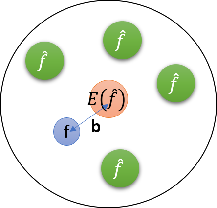
Figure 1: The schematic drawing of bias and variance.

3 Empirical cumulative distribution function

Given a sample \(x_1, x_2, \cdots, x_n\) with a common cumulative distribution function \(F\), for example the calculated work for a given pulling rate in the pulling experiment, the empirical cumulative distribution function is defined as

\[\begin{equation} \hat{F}_n(t) = \frac{number\, of\, elements\, \leq t}{n} \equiv \frac{1}{n}\sum_{i=1}^{n}\pmb{I}_{(-\infty, t)}(x_i) \label{eq:cdfd} \end{equation}\]

where \(\pmb{I}\) is the indicator function. An indicator function of a subset \(A\) of a set \(X\) is a binary function from \(X\) to \(\{0, 1\}\) defined as

\[ \pmb{I}_A(x) := \begin{cases} 1 & x\in A \\ 0 & x\notin A \end{cases} \]

To plot the empirical cumulative function, we first arrange the \(n\) sample points in ascending order to get \(x_{(1)}, x_{(2)}, \cdots, x_{(n)}\), allowing repeated numbers. Then the empirical cumulative function is a step function that jumps by \(1/n\) at each sample point: \((x_{(1)}, x_{(2)}, \cdots, x_{(n)}) \rightarrow (\frac{1-0.5}{n}, \frac{2-0.5}{n}, \cdots, \frac{n-0.5}{n})\).

Example. A sample consists of ten observations: \(176, 192, 214, 220, 205, 192, 201, 192, 183, 185\). The following chunk plot its empirical cumulative function.

x <- c(176, 192, 214, 220, 205, 192, 201, 192, 183, 185)
n <- length(x)
plot(sort(x), ((1:n) - 0.5)/n, type = 's', ylim = c(0, 1), xlab = 'x: observations', ylab = '', main = 'Empirical Cumulative Distribution')
# add the label on the y-axis
mtext(text = expression(hat(F)[n](x)), side = 2, line = 2.5)

4 Density function estimated from histogram

Since it is natural to treat a rescaled histogram as the estimation of a probability density function, we give a mathematical derivation on the rescaled histograms.

Figure 2: The schematic drawing of a histogram.

Given \(n\) sample points \(\pmb{x}\) and \(M\) bins shown in Figure 2, what is the maximum probability of observing \(n_i\) sample points in the \(i\)th bin? Assume that the probability of observing one sample point in the \(i\)th bin is \(c_i\), the problem is to find optimal \(c_i^*\) to maximize

\[\begin{equation} \mathcal{L}(\pmb{x} \mid \pmb{c}) = \prod_{i=1}^{M}p(n_i \mid c_i) = \prod_{i=1}^{M}c_i^{n_i} \label{eq:cost} \end{equation}\]

The optimization is subject to the density function constraint:

\[\begin{equation} \sum_{i=1}^{M}c_i w_i = 1 \label{eq:constraint} \end{equation}\]

where \(w_i\) is the width of the \(i\)th bin.

Using the method of Lagrange multipliers, the problem can be converted to find optimal \(c_i^*\) to minimize

\[\begin{equation} \begin{split} f(\pmb{c}) & = \log (\prod_{i=1}^{M}c_i^{n_i}) - \lambda (\sum_{i=1}^{M}c_i w_i - 1) \\ & = \sum_{i=1}^{M}n_i \log c_i - \lambda (\sum_{i=1}^{M}c_i w_i - 1) \end{split} \label{eq:lagrange} \end{equation}\]

Here we have taken the log of the cost function (\ref{eq:cost}) so we can deal with sums rather than products. Computing the derivatives and using the constraints, we can find that \(\lambda = n\) and \(c_i^*=\frac{n_i}{n w_i}\).

5 Error estimate

As shown in Section 3, the density of \(x\) in a bin \(b \equiv (x_0, x_0 +h]\) is

\[\begin{equation} \hat{f}_n(x) = \frac{1}{hn}\sum_{i=1}^{n}\pmb{I}_{(x_0, x_0 + h]}(x_i) \label{eq:density} \end{equation}\]

The sum in Equation (\ref{eq:density}) is actually the number of points in the bin \(b\). It is a bionomial random variable \(B \sim Binomial(n, p)\), where \(p\) is the probability of one point falling into the bin \(p = F(x_0 + h) - F(x_0)\). The Binomial distribution tells that the mean and variance of \(B\) is \(np\) and \(np(1-p)\), respectively. So the mean of \(\hat{f}_n(x)\) is

\[\begin{equation} \begin{split} \mathbb{E}\left[ \hat{f}_n(x) \right] & = \frac{1}{nh} \mathbb{E}[B] \\ & = \frac{n [F(x_0 + h) - F(x_0)]}{nh} \\ & = \frac{[F(x_0 + h) - F(x_0)]}{h} \\ & = f(x^*) \end{split} \label{eq:mean} \end{equation}\]

The last equality in Equation (\ref{eq:mean}) is due to the mean value theorem. It implies that if we use smaller and smaller bins as we get more data, the histogram density estimate is unbiased.

The variance of \(\hat{f}_n(x)\) is

\[\begin{equation} \begin{split} \mathbb{V}\left[ \hat{f}_n(x) \right] & = \frac{1}{n^2 h^2} \mathbb{V}\left[ B \right]\\ & = \frac{n[F(x_0 + h) - F(x_0)][1 - F(x_0 + h) + F(x_0)]}{n^2 h^2} \\ & = \frac{nhf(x^*)(1-hf(x^*))}{n^2 h^2} \\ & = \frac{f(x^*)}{nh} - \frac{f(x^*)^2}{n} \end{split} \label{eq:vari} \end{equation}\]

Therefore, the mean squared error (MSE) between the true and estimated density \(\hat{f}_n (x)\) is

\[\begin{equation} \begin{split} \mathbb{E}[(f(x)-\hat{f}_n (x))^2] & = (\mathbb{E}[\hat{f}_n (x)] - f(x))^2 + \mathbb{V}[\hat{f}_n(x)] \\ & = (f'(x^{**})(x^{*}-x))^2 + \frac{f(x^*)}{nh} - \frac{f(x^*)^2}{n} \\ & \leq (Lh)^2 + \frac{f(x^*)}{nh} - \frac{f(x^*)^2}{n} \end{split} \label{eq:msef} \end{equation}\]

where \(L = \underset{x\in [x_0, x_0 + h]}{\max}f'(x)\). Equation (\ref{eq:mse}) implies that the error depends on the choices of bin size \(h\) and the data size. The minimum error bound is reached when

\[\begin{equation} h = \left(\frac{f(x^{*})}{2L^2 n}\right)^{1/3} \label{eq:h} \end{equation}\]

Since \(L\) and \(f(x^{*})\) are unknown, it is an art to choose the right \(h\). The Scott’s rule (1979) sets \(h = 3.5 s n^{-1/3}\), where \(s\) is the sample standard deviation. The Freedman and Diaconis’s (1981) rule sets \(h = 2(IQ)n^{-1/3}\), where \(IQ\) is the sample interquartile range. In R, the default rule is the Sturges’ rule which set the number of bins as \(1 + \log_{2} n\).

6 References

Scott, D.W.(1979) On optimal and data-based histograms. Biometrika, 66, 605–610.

Freedman, D.andDiaconis, P.(1981) On this histogram as a density estimator:L2theory. Zeit. Wahr. ver. Geb.,57, 453–476.

Sturges, H.(1926) The choice of a class-interval.J. Amer. Statist. Assoc., 21, 65–66.

Myles Hollander, Douglas A. Wolfe, Eric Chicken. (2014) Nonparametric Statistical Methods, Third Edition. John Wiley & Sons, Inc.